Download a copy of the vignette to follow along here: a_simple_example.Rmd
In this vignette, we will show how metasnf can be used
for a very simple SNF workflow.
This simple workflow is the example of SNF provided in the original
SNFtool package. You can find the example by loading the
SNFtool package and then viewing the documentation for the main
SNF function by running ?SNF.
The original SNF example
1. Load the package
library(SNFtool)2. Set SNF hyperparameters
Three hyperparameters are introduced in this example: K, alpha (also referred to as sigma or eta in different documentations), and T. You can learn more about the significance of these hyperparameters in the original SNF paper (see references).
K <- 20
alpha <- 0.5
T <- 20
3. Load the data
The SNFtool package provides two mock data frames titled Data1 and Data2 for this example. Data1 contains gene expression values of two genes for 200 patients. Data2 similarly contains methylation data for two genes for those same 200 patients.
Here’s what the mock data looks like:
library(ComplexHeatmap)

# gene expression data
gene_expression_hm <- Heatmap(
    as.matrix(Data1),
    cluster_rows = FALSE,
    cluster_columns = FALSE,
    show_row_names = FALSE,
    show_column_names = FALSE,
    heatmap_legend_param = list(
        title = "Gene Expression"
    )
)

gene_expression_hm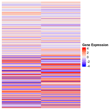
# methylation data
methylation_hm <- Heatmap(
    as.matrix(Data2),
    cluster_rows = FALSE,
    cluster_columns = FALSE,
    show_row_names = FALSE,
    show_column_names = FALSE,
    heatmap_legend_param = list(
        title = "Methylation"
    )
)

methylation_hm
The “ground truth” of how this data was generated was that patients 1 to 100 were drawn from one distribution and patients 101 to 200 were drawn from another. We don’t have access to that kind of knowledge in real data, but we do here.
4. Generate similarity matrices for each data source
We consider the two gene expression features in Data1 to contain information from one broader gene expression source and the two methylation features in Data2 to contain information from a broader methylation source.
The next step is to determine, for each of the sources we have, how similar all of our patients are to each other.
This is done by first determining how dissimilar the patients are to each other for each source, and then converting that dissimilarity information into similarity information.
To calculate dissimilarity, we’ll use Euclidean distance.
distance_matrix_1 <- as.matrix(dist(Data1, method = "euclidean"))
distance_matrix_2 <- as.matrix(dist(Data2, method = "euclidean"))
Then, we can use the affinityMatrix function provided by
SNFtool to convert those distance matrices into similarity
matrices.
similarity_matrix_1 <- affinityMatrix(distance_matrix_1, K, alpha)
similarity_matrix_2 <- affinityMatrix(distance_matrix_2, K, alpha)
Those similarity matrices can be passed into the SNF
function to integrate them into a single similarity matrix that
describes how similar the patients are to each other across both the
gene expression and methylation data.
6. Find clusters in the integrated matrix
If we think there are 2 clusters in the data, we can use spectral clustering to find 2 clusters in the fused network.
number_of_clusters <- 2
assigned_clusters <- spectralClustering(fused_network, number_of_clusters)
Sure enough, we are able to obtain the correct cluster label for all patients.
all(true_label == assigned_clusters)
#> [1] TRUE
The same example using metasnf
The purpose of metasnf is primarily to aid users explore
a wide possible range of solutions. Recreating the example provided with
the original SNF function will be an extremely restricted
usage of the package, but will reveal, broadly, how metasnf
works.
2. Store the data in a data list
Data used for clustering will be stored in a data_list
class object. The data list is made by passing each data frame into the
data_list() function, alongside information about the name
of the data frame, the broader source (referred to in this package as a
“domain”) of information that data frame comes from, and the type of
features that are stored inside that data frame (can be continuous,
discrete, ordinal, categorical, or mixed). The data_list()
function also requires you to specify which column contains information
about the ID of the patients. In this case, that information isn’t
there, so we’ll have to add it ourselves. The added IDs span from 101
onwards (rather than from 1 onwards) purely for convenience: automatic
sorting of patient names won’t result in patient 199 being placed before
patient 2.
# Add "patient_id" column to each data frame
Data1$"patient_id" <- 101:(nrow(Data1) + 100)
Data2$"patient_id" <- 101:(nrow(Data2) + 100)

my_dl <- data_list(
    list(
        data = Data1,
        name = "genes_1_and_2_exp",
        domain = "gene_expression",
        type = "continuous"
    ),
    list(
        data = Data2,
        name = "genes_1_and_2_meth",
        domain = "gene_methylation",
        type = "continuous"
    ),
    uid = "patient_id"
)
The entries are lists which contain the following elements:
- The data frame
- A user-determined name for the data frame (character)
- A user-determined name for the domain of information the data frame is representative of (character)
- The type of feature stored in the data frame (character; options are continuous, discrete, ordinal, categorical, and mixed)
Finally, there’s an argument for the uid (the column
name that currently uniquely identifies all the observations in your
data).
In the process of formatting the provided data frames, this function:
- Converts the UID of the data into “uid”
- Prefixing the UID values with the string “uid_” to help with cluster result characterization
- Removes all observations that contain any missing values
- Removes all observations that are not present in all data frames
- Arranges the observations in all data frames by their UID
To avoid losing a considerable amount of data during data list
generation, consider using imputation
first. The mice package in R is helpful for this.
Also note that you do not need to name out every element explicitly; as long as you provide the objects within each list in the correct order (data, name, domain, type), you’ll get the correct result:
3. Store all the settings of the desired SNF runs in an SNF config
The SNF config is an object storing all the information required to convert the raw data into a final cluster solution. It is composed of multiple parts, including a settings data frame which tracks one set of SNF hyperparameters per row, a weights matrix which tracks one set of all the feature weights per row, a distance functions list which stores all the functions that will be uesd to convert raw data into a intermediate distance matrices, and a clustering algorithms list which stores all the functions that will be used to convert final SNF-fused networks into cluster solutions. By varying the elements in the SNF config, we can access a broader space of possible solutions and hopefully get closer to something that will be as useful as possible for our context.
In this case, we’re going to create only a single cluster solution using the same process outlined in the original SNFtool example above.
A full explanation of all the parameters in the
snf_config() function can be found at the
SNF config vignette.
sc <- snf_config(
    dl = my_dl,
    n_solutions = 1,
    alpha_values = 0.5,
    k_values = 20,
    t_values = 20,
    dropout_dist = "none",
    possible_snf_schemes = 1
)
#> ℹ No distance functions specified. Using defaults.
#> ℹ No clustering functions specified. Using defaults.

sc
#> Settings Data Frame:
#>                         1
#> SNF hyperparameters:
#> alpha                 0.5
#> k                      20
#> t                      20
#> SNF scheme:
#>                         1
#> Clustering functions:
#>                         2
#> Distance functions:
#> CNT                     1
#> DSC                     1
#> ORD                     1
#> CAT                     1
#> MIX                     1
#> Component dropout:
#> genes_1_and_2_exp       ✔
#> genes_1_and_2_meth      ✔
#> Distance Functions List:
#> Continuous (1):
#> [1] euclidean_distance
#> Discrete (1):
#> [1] euclidean_distance
#> Ordinal (1):
#> [1] euclidean_distance
#> Categorical (1):
#> [1] gower_distance
#> Mixed (1):
#> [1] gower_distance
#> Clustering Functions List:
#> [1] spectral_eigen
#> [2] spectral_rot
#> Weights Matrix:
#> Weights defined for 1 cluster solutions.
#> $ V1  1
#> $ V2  1
#> $ V3  1
#> $ V4  1
We can more clearly examine the settings data frame within the config as follows:
as.data.frame(sc$"settings_df")
#>   solution alpha  k  t snf_scheme clust_alg cnt_dist dsc_dist ord_dist cat_dist
#> 1        1   0.5 20 20          1         2        1        1        1        1
#>   mix_dist inc_genes_1_and_2_exp inc_genes_1_and_2_meth
#> 1        1                     1                      1
The columns in this settings_df-class object account for
the following:
- solution: A way to keep track of the different rows
- alpha, k, t: The hyperparameters seen above
- snf_scheme: Which “scheme” will be used to transform the inputs into a final fused network. We’ll discuss this in more detail in the next vignette.
- clust_alg: Which clustering function from the
clust_fns_listwill be applied to the final fused network. By default, theclust_fns_listhas index 1 referencing spectral clustering paired with the eigen-gap heuristic determining the number of clusters, while index 2 references spectral clustering paired with the rotation cost heuristic instead. - Columns ending in “dist”: Which distance metric function from the
dist_fns_listshould be used. By default, thedist_fns_listhas index 1 referencing simple Euclidean distance for continuous, discrete, and ordinal data, and Gower’s distance for categorical and mixed data. - Columns starting with “inc”: Component dropout - whether or not the corresponding data frame will be included for this round of SNF.
More detailed descriptions on all of these columns can also be found in the the SNF config vignette.
4. Run SNF
The batch_snf function will use all of the
hyperparameters and functions stored in the SNF config to the create
cluster solutions from the data_list.
sol_df <- batch_snf(dl = my_dl, sc = sc)

sol_df
#> 1 cluster solution of 200 observations:
#> solution nclust mc uid_101 uid_102 uid_103 uid_104 uid_105 uid_106 uid_107
#>        1      2  .       1       1       1       1       1       1       1
#> 193 observations not shown.
#> Use `print(n = ...)` to change the number of rows printed.
#> Use `t()` to view compact cluster solution format.
The solutions data frame (solutions_df class object) is
a data frame that contains one cluster solution per row. essentially an
augmented , where new columns have been added for each included patient.
On each row, those new columns show what cluster that patient ended up
in.
A friendlier format of the clustering results can be obtained:
cluster_solution <- t(sol_df)

cluster_solution
#> 1 cluster solution of 200 observations:
#>     uid      s1
#> uid_101       1
#> uid_102       1
#> uid_103       1
#> uid_104       1
#> uid_105       1
#> uid_106       1
#> uid_107       1
#> uid_108       1
#> uid_109       1
#> uid_110       1
#> 190 observations not shown.
These cluster results are exactly the same as in the original SNF example:
all.equal(cluster_solution$"s1", true_label)
#> [1] TRUE
Running batch_snf with the return_sim_mats
parameter set to TRUE will let us also take a look at the
final fused networks from SNF rather than just the results of applying
spectral clustering to those networks:
sol_df <- batch_snf(
    dl = my_dl,
    sc,
    return_sim_mats = TRUE
)

# The first (and only, in this case) final fused network
similarity_matrix <- sim_mats_list(sol_df)[[1]]
The fused network obtained through this approach is also the same as the one obtained in the original example:
max(similarity_matrix - fused_network)
#> [1] 0
And now we’ve completed a basic example of using this package. The subsequent vignettes provide guidance on how you can leverage the SNF config to access a wide range of clustering solutions from your data, how you can use other tools in this package to pick a best solution for your purposes, and how to validate the generalizability of your results.
Go give the less simple example a try!
References
Wang, Bo, Aziz M. Mezlini, Feyyaz Demir, Marc Fiume, Zhuowen Tu, Michael Brudno, Benjamin Haibe-Kains, and Anna Goldenberg. 2014. “Similarity Network Fusion for Aggregating Data Types on a Genomic Scale.” Nature Methods 11 (3): 333–37. https://doi.org/10.1038/nmeth.2810.