Download a copy of the vignette to follow along here: a_complete_example.Rmd
We recommend you go through the simple example before working through this one.
This vignette walks through how the core functionality of this package, including:
- Setting up the data
- Building a space of settings to cluster over
- Running SNF
- Identifying and visualizing meta clusters
- Characterizing and selecting top meta clusters
- Selecting a representative cluster solution from a meta cluster
- Cluster solution characterization
- Cluster solution validation
Data Set-up
Pre-processing
Your data should be loaded into the R environment in the following format:
- The data is in one or more
data.frameclass objects - The data is in wide form (one row per observation to cluster)
- All data frames should have exactly one column that uniquely identifies each observation
- All data should be complete (no missing values)
If you wish to use imputation to handle missingness in your data, you can take a look at the imputation vignette which outlines a basic workflow for meta clustering across multiple imputations of the same dataset.
The package comes with a few mock data frames based on real data from the Adolescent Brain Cognitive Development study:
-
anxiety(anxiety scores from the CBCL) -
depress(depression scores from the CBCL) -
cort_t(cortical thicknesses) -
cort_sa(cortical surface areas in mm^2) -
subc_v(subcortical volumes in mm^3) -
income(household income on a 1-3 scale) -
pubertal(pubertal status on a 1-5 scale)
Here’s what the cortical thickness data looks like:
library(metasnf)

class(cort_t)
#> [1] "tbl_df"     "tbl"        "data.frame"

dim(cort_t)
#> [1] 188 152

str(cort_t[1:5, 1:5])
#> Classes 'tbl_df', 'tbl' and 'data.frame':    5 obs. of  5 variables:
#>  $ unique_id: chr  "NDAR_INV0567T2Y9" "NDAR_INV0GLZNC2W" "NDAR_INV0IZ157F8" "NDAR_INV0J4PYA5F" ...
#>  $ mrisdp_1 : num  2.6 2.62 2.62 2.6 2.53
#>  $ mrisdp_2 : num  2.49 2.85 2.29 2.67 2.76
#>  $ mrisdp_3 : num  2.8 2.78 2.53 2.68 2.83
#>  $ mrisdp_4 : num  2.95 2.85 2.96 2.94 2.99

cort_t[1:5, 1:5]
#>          unique_id mrisdp_1 mrisdp_2 mrisdp_3 mrisdp_4
#> 1 NDAR_INV0567T2Y9    2.601    2.487    2.801    2.954
#> 2 NDAR_INV0GLZNC2W    2.619    2.851    2.784    2.846
#> 3 NDAR_INV0IZ157F8    2.621    2.295    2.530    2.961
#> 4 NDAR_INV0J4PYA5F    2.599    2.670    2.676    2.938
#> 5 NDAR_INV0OYE291Q    2.526    2.761    2.829    2.986
The first column unique_id is the unique identifier
(UID) for all observations in the data.
Here’s the household income data:
dim(income)
#> [1] 275   2

str(income[1:5, ])
#> Classes 'tbl_df', 'tbl' and 'data.frame':    5 obs. of  2 variables:
#>  $ unique_id       : chr  "NDAR_INV0567T2Y9" "NDAR_INV0GLZNC2W" "NDAR_INV0IZ157F8" "NDAR_INV0J4PYA5F" ...
#>  $ household_income: num  3 NA 1 2 1

income[1:5, ]
#>          unique_id household_income
#> 1 NDAR_INV0567T2Y9                3
#> 2 NDAR_INV0GLZNC2W               NA
#> 3 NDAR_INV0IZ157F8                1
#> 4 NDAR_INV0J4PYA5F                2
#> 5 NDAR_INV0OYE291Q                1
Putting everything in a list will help us get quicker summaries of all the data.
df_list <- list(
    anxiety,
    depress,
    cort_t,
    cort_sa,
    subc_v,
    income,
    pubertal
)

# The number of rows in each data frame:
lapply(df_list, dim)
#> [[1]]
#> [1] 275   2
#>
#> [[2]]
#> [1] 275   2
#>
#> [[3]]
#> [1] 188 152
#>
#> [[4]]
#> [1] 188 152
#>
#> [[5]]
#> [1] 174  31
#>
#> [[6]]
#> [1] 275   2
#>
#> [[7]]
#> [1] 275   2

# Whether or not each data frame has missing values:
lapply(df_list,
    function(x) {
        any(is.na(x))
    }
)
#> [[1]]
#> [1] TRUE
#>
#> [[2]]
#> [1] TRUE
#>
#> [[3]]
#> [1] FALSE
#>
#> [[4]]
#> [1] FALSE
#>
#> [[5]]
#> [1] FALSE
#>
#> [[6]]
#> [1] TRUE
#>
#> [[7]]
#> [1] TRUE
Some of the data has missing values and not all of the data frames
have the same number of participants. SNF can only be run with complete
data, so you’ll need to either use complete case analysis (removal of
observations with any missing values) or impute the missing values to
proceed with the clustering. As mentioned above, metasnf
can be used to visualize changes in clustering results across different
imputations of the data.
For now, we’ll just examine the simpler complete-case analysis
approach by reducing our data frames to only common and complete
observations. This can be made easier using the
get_complete_uids function.
complete_uids <- get_complete_uids(df_list, uid = "unique_id")

print(length(complete_uids))
#> [1] 87

# Reducing data frames to only common observations with no missing data
anxiety <- anxiety[anxiety$"unique_id" %in% complete_uids, ]
depress <- depress[depress$"unique_id" %in% complete_uids, ]
cort_t <- cort_t[cort_t$"unique_id" %in% complete_uids, ]
cort_sa <- cort_sa[cort_sa$"unique_id" %in% complete_uids, ]
subc_v <- subc_v[subc_v$"unique_id" %in% complete_uids, ]
income <- income[income$"unique_id" %in% complete_uids, ]
pubertal <- pubertal[pubertal$"unique_id" %in% complete_uids, ]
Generating the data list
The data_list class is a structured list of data frames
(like the one already created), but with some additional metadata about
each data frame. It should only contain the data frames we want to
directly use as inputs for the clustering. Let’s say we are working in a
context where the anxiety and depression data are especially important
outcomes and we want to know if we can find subtypes using the other
data which still do a good job of separating out observations by their
anxiety and depression scores.
We’ll start by initializing a data list that stores our input features.
# Note that you do not need to explicitly name every single named element
# (data = ..., name = ..., etc.)
input_dl <- data_list(
    list(
        data = cort_t,
        name = "cortical_thickness",
        domain = "neuroimaging",
        type = "continuous"
    ),
    list(
        data = cort_sa,
        name = "cortical_surface_area",
        domain = "neuroimaging",
        type = "continuous"
    ),
    list(
        data = subc_v,
        name = "subcortical_volume",
        domain = "neuroimaging",
        type = "continuous"
    ),
    list(
        data = income,
        name = "household_income",
        domain = "demographics",
        type = "continuous"
    ),
    list(
        data = pubertal,
        name = "pubertal_status",
        domain = "demographics",
        type = "continuous"
    ),
    uid = "unique_id"
)
This process removes any observations that did not have complete data across all provided input data frames. The structure of the data list is a nested list tracking the data, the name of the data frame, what domain (broader source of information) the data frame belongs to, and the type of feature stored in that data frame. Options for feature type include “continuous”, “discrete”, “ordinal”, “categorical”, and “mixed”.
The uid parameter is the name of the column in the data
frames that uniquely identifies each observation. Upon data list
creation, the UID will be converted to "uid" and the UIDs
themselves will be prefixed with "_uid" for ease of
management across other functions in the package.
We can get a summary of our constructed data list with the
summary function:
summary(input_dl)
#>                    name       type       domain length width
#> 1    cortical_thickness continuous neuroimaging     87   151
#> 2 cortical_surface_area continuous neuroimaging     87   151
#> 3    subcortical_volume continuous neuroimaging     87    30
#> 4      household_income continuous demographics     87     1
#> 5       pubertal_status continuous demographics     87     1
Each input data frame now has the same 87 observations with complete data. The width refers to the number of features in each data frame (not including the UID column).
data_list now stores all the features we intend on using
for the clustering. We’re interested in knowing if any of the clustering
solutions we generate can distinguish children apart based on their
anxiety and depression scores. To do this, we’ll also create a data list
storing only features that we’ll use for evaluating our cluster
solutions and not for the clustering itself. We’ll refer to this as the
target data list.
target_dl <- data_list(
    list(anxiety, "anxiety", "behaviour", "ordinal"),
    list(depress, "depressed", "behaviour", "ordinal"),
    uid = "unique_id"
)

summary(target_dl)
#>        name    type    domain length width
#> 1   anxiety ordinal behaviour     87     1
#> 2 depressed ordinal behaviour     87     1
Note that it is not necessary to make use of a partition of input and out-of-model measures in this way. If you’d like to have no target data list and instead use every single feature of interest for the clustering, you can stick to just using one data list.
Defining sets of hyperparameters to use for SNF and clustering
The SNF config stores all the information about the settings and
functions to be used for each SNF run to be completed. Calling the
snf_config function with a specified number of rows will
automatically build a randomly populated snf_config class
object.
set.seed(42)
my_sc <- snf_config(
    dl = input_dl,
    n_solutions = 20,
    min_k = 20,
    max_k = 50
)
#> ℹ No distance functions specified. Using defaults.
#> ℹ No clustering functions specified. Using defaults.

my_sc
#> Settings Data Frame:
#>                            1    2    3    4    5    6    7    8    9   10
#> SNF hyperparameters:
#> alpha                    0.5  0.4  0.3  0.3  0.5  0.4  0.7  0.8  0.3  0.6
#> k                         29   26   44   43   29   26   36   21   29   35
#> t                         20   20   20   20   20   20   20   20   20   20
#> SNF scheme:
#>                            2    1    2    1    2    2    2    3    1    3
#> Clustering functions:
#>                            1    1    2    1    2    1    1    2    1    1
#> Distance functions:
#> CNT                        1    1    1    1    1    1    1    1    1    1
#> DSC                        1    1    1    1    1    1    1    1    1    1
#> ORD                        1    1    1    1    1    1    1    1    1    1
#> CAT                        1    1    1    1    1    1    1    1    1    1
#> MIX                        1    1    1    1    1    1    1    1    1    1
#> Component dropout:
#> cortical_thickness         ✔    ✔    ✔    ✔    ✔    ✔    ✔    ✔    ✔    ✔
#> cortical_surface_area      ✖    ✔    ✖    ✔    ✔    ✔    ✔    ✔    ✔    ✔
#> subcortical_volume         ✔    ✔    ✖    ✖    ✔    ✔    ✔    ✔    ✔    ✔
#> household_income           ✖    ✔    ✔    ✔    ✔    ✔    ✔    ✖    ✔    ✖
#> pubertal_status            ✔    ✔    ✔    ✔    ✔    ✔    ✔    ✔    ✔    ✖
#> …and settings defined to create 10 more cluster solutions.
#> Distance Functions List:
#> Continuous (1):
#> [1] euclidean_distance
#> Discrete (1):
#> [1] euclidean_distance
#> Ordinal (1):
#> [1] euclidean_distance
#> Categorical (1):
#> [1] gower_distance
#> Mixed (1):
#> [1] gower_distance
#> Clustering Functions List:
#> [1] spectral_eigen
#> [2] spectral_rot
#> Weights Matrix:
#> Weights defined for 20 cluster solutions.
#> $ mrisdp_1 1, 1, 1, 1, 1, 1, 1, 1, 1, 1, 1, 1, 1, 1, 1…
#> $ mrisdp_2 1, 1, 1, 1, 1, 1, 1, 1, 1, 1, 1, 1, 1, 1, 1…
#> $ mrisdp_3 1, 1, 1, 1, 1, 1, 1, 1, 1, 1, 1, 1, 1, 1, 1…
#> $ mrisdp_4 1, 1, 1, 1, 1, 1, 1, 1, 1, 1, 1, 1, 1, 1, 1…
#> $ mrisdp_5 1, 1, 1, 1, 1, 1, 1, 1, 1, 1, 1, 1, 1, 1, 1…
#> …and 329 more features.
The SNF config contains multiple parts that all play a role in determining how the data in a data list will be converted into a cluster solution.
The settings data frame
The first part is the settings data frame:
my_sc$"settings_df"
#>                            1    2    3    4    5    6    7    8    9   10
#> SNF hyperparameters:
#> alpha                    0.5  0.4  0.3  0.3  0.5  0.4  0.7  0.8  0.3  0.6
#> k                         29   26   44   43   29   26   36   21   29   35
#> t                         20   20   20   20   20   20   20   20   20   20
#> SNF scheme:
#>                            2    1    2    1    2    2    2    3    1    3
#> Clustering functions:
#>                            1    1    2    1    2    1    1    2    1    1
#> Distance functions:
#> CNT                        1    1    1    1    1    1    1    1    1    1
#> DSC                        1    1    1    1    1    1    1    1    1    1
#> ORD                        1    1    1    1    1    1    1    1    1    1
#> CAT                        1    1    1    1    1    1    1    1    1    1
#> MIX                        1    1    1    1    1    1    1    1    1    1
#> Component dropout:
#> cortical_thickness         ✔    ✔    ✔    ✔    ✔    ✔    ✔    ✔    ✔    ✔
#> cortical_surface_area      ✖    ✔    ✖    ✔    ✔    ✔    ✔    ✔    ✔    ✔
#> subcortical_volume         ✔    ✔    ✖    ✖    ✔    ✔    ✔    ✔    ✔    ✔
#> household_income           ✖    ✔    ✔    ✔    ✔    ✔    ✔    ✖    ✔    ✖
#> pubertal_status            ✔    ✔    ✔    ✔    ✔    ✔    ✔    ✔    ✔    ✖
#> …and settings defined to create 10 more cluster solutions.
The settings data frame stores information about:
-
SNF hyperparameters:
alpha,k, andthyperparameters that are directly used by the SNF algorithm. - SNF scheme: the specific way in which input data gets collapsed into a final fused network (discussed further in the SNF schemes vignette).
- Clustering functions: Which clustering algorithm will be applied to the final fused network produced by SNF.
- Distance function: Which distance metric will be used when converting continuous, discrete, ordinal, categorical, or mixed type data into intermediate distance matrices (discussed further in the distance metrics vignette).
- Component dropout - Information on whether or not a particular input data frame in the data list will be in included or excluded from the corresponding SNF run (discussed further in the SNF config vignette).
The underlying structure of a settings data frame can be viewed by
converting it from a settings_df class object into a
regular data.frame class object:
head(as.data.frame(my_sc$"settings_df"))
#>   solution alpha  k  t snf_scheme clust_alg cnt_dist dsc_dist ord_dist cat_dist
#> 1        1   0.5 29 20          2         1        1        1        1        1
#> 2        2   0.4 26 20          1         1        1        1        1        1
#> 3        3   0.3 44 20          2         2        1        1        1        1
#> 4        4   0.3 43 20          1         1        1        1        1        1
#> 5        5   0.5 29 20          2         2        1        1        1        1
#> 6        6   0.4 26 20          2         1        1        1        1        1
#>   mix_dist inc_cortical_thickness inc_cortical_surface_area
#> 1        1                      1                         0
#> 2        1                      1                         1
#> 3        1                      1                         0
#> 4        1                      1                         1
#> 5        1                      1                         1
#> 6        1                      1                         1
#>   inc_subcortical_volume inc_household_income inc_pubertal_status
#> 1                      1                    0                   1
#> 2                      1                    1                   1
#> 3                      0                    1                   1
#> 4                      0                    1                   1
#> 5                      1                    1                   1
#> 6                      1                    1                   1
Each row of the settings data frame corresponds to a set of
hyperparameters that can be used for generating a cluster solution.
Without specifying any additional parameters, the
snf_config function randomly populates these columns and
ensures that no generated rows are identical. Further customization of
the settings_df and the other parts of the SNF config will
enable you to generate a broader space of cluster solutions from your
data and ideally get you closer to finding a more useful solution for
your context. More on settings_df customization can be
found in the SNF
config vignette.
Setting a seed prior to calling snf_config() ensures
that the same random settings are generated each time we run the
code.
Other parts of the SNF config
There are three other parts to an SNF config object: a distance
functions list (dist_fns_list class object) that stores
distance metric functions, a clustering functions list
(clust_fns_list class object) that stores clustering
algorithm functions, and a weights matrix (weights_matrix)
class object that stores feature weights.
names(my_sc)
#> [1] "settings_df"    "dist_fns_list"  "clust_fns_list" "weights_matrix"
Customizing each of these parts is explained in more detail in separate vignettes:
For now, we’ll leave them as the default values generated during our
snf_config call.
Running SNF and clustering
The batch_snf() function integrates the data in the data
list using all the hyperparameters, and functions contained in the SNF
config. The resulting structure is a solutions_df class
object, which contains an index column (solution), a column
tracking the number of clusters in the cluster solution
(nclust), a column labeling which meta cluster a solution
belongs to (mc; more on this later) and columns specifying
which cluster each subject was assigned to for each corresponding
solution.
sol_df <- batch_snf(input_dl, my_sc)

sol_df
#> 20 cluster solutions of 87 observations:
#> solution nclust mc uid_NDAR_INV0567T2Y9 uid_NDAR_INV0J4PYA5F
#> 1 5 . 5 2
#> 2 3 . 3 3
#> 3 9 . 1 7
#> 4 2 . 1 2
#> 5 8 . 1 6
#> 6 2 . 1 2
#> 7 4 . 1 4
#> 8 5 . 3 4
#> 9 3 . 3 3
#> 10 4 . 2 4
#> 10 solutions and 85 observations not shown.
#> Use `print(n = ...)` to change the number of rows printed.
#> Use `t()` to view compact cluster solution format.Just like that, 20 different cluster solutions have been generated!
In practice, you may end up wanting to create hundreds or thousands of
cluster solutions at a time. If you have access to a multi-core system,
batch_snf can be run with parallel processing enabled. See
?batch_snf or the parallel
processing vignette for more information.
You can pull the clustering results out of each row in a more
convenient, transposed format using the t() function:
cluster_solutions <- t(sol_df)

cluster_solutions
#> 20 cluster solutions of 87 observations:
#>                  uid      s1    s2    s3    s4    s5    s6    s7    s8    s9
#> uid_NDAR_INV0567T2Y9       5     3     1     1     1     1     1     3     3
#> uid_NDAR_INV0J4PYA5F       2     3     7     2     6     2     4     4     3
#> uid_NDAR_INV10OMKVLE       1     2     3     1     4     2     3     1     2
#> uid_NDAR_INV15FPCW4O       1     2     5     2     5     2     3     1     2
#> uid_NDAR_INV19NB4RJK       4     2     9     1     7     2     3     2     2
#> uid_NDAR_INV1HLGR738       4     2     9     1     7     2     3     2     2
#> uid_NDAR_INV1KR0EZFU       4     2     9     1     7     2     3     2     2
#> uid_NDAR_INV1L3Y9EOP       1     2     5     2     5     2     3     1     2
#> uid_NDAR_INV1TCP5GNM       1     2     3     1     4     2     3     1     2
#> uid_NDAR_INV1ZHRDJ6B       3     1     4     1     7     1     3     5     2
#> 11 solutions and 77 observations not shown.
When transposed, the solutions_df class object is
converted to a t_solutions_df class object, which only
contains columns indicating what cluster each observation was assigned
to for each solution. Calling t() on a
t_solutions_df class object will return it back to its
original solutions_df form.
Identifying and visualizing meta clusters
Now that we have access to 20 different clustering solutions, we’ll need to find some way to pick an optimal one to move forward with for additional characterization. In this case, plotting or running stats manually on each of the solutions might be a reasonable way to determine which ones may be the most suitable for our purpose. But when the number of solutions generated goes up into the hundreds (or thousands), these approaches can become impractical or inefficient.
The main approach we recommend using is the meta clustering approach described in Caruana et al., 2006. Meta clustering is a useful approach when the criteria for cluster solution evaluation is difficult to formalize and fully automate. Meta clustering consists of clustering the clustering solutions themselves to yield a manageable number of qualitatively similar meta cluster solutions that are representative of the full set of solutions. Characterization of these representative solutions then enables efficient identification of a maximally useful cluster solution for the user’s context.
The first step in meta clustering is to calculate the adjusted Rand index (ARI) between each pair of cluster solutions. This metric tells us how similar the solutions are to each other, thereby allowing us to find clusters of cluster solutions.
sol_aris <- calc_aris(sol_df)

head(sol_aris)
#>              1           2          3           4         5            6
#> 1  1.000000000 0.207544990 0.35774499  0.09280937 0.3341715 -0.007786117
#> 2  0.207544990 1.000000000 0.11544848  0.36498713 0.1039936  0.005037111
#> 3  0.357744993 0.115448475 1.00000000  0.09394738 0.9217495  0.151933583
#> 4  0.092809374 0.364987135 0.09394738  1.00000000 0.1058439 -0.010286490
#> 5  0.334171519 0.103993559 0.92174950  0.10584388 1.0000000  0.143121635
#> 6 -0.007786117 0.005037111 0.15193358 -0.01028649 0.1431216  1.000000000
#>           7            8            9           10         11        12
#> 1 0.3095424  0.984996843  0.173570236 -0.008291469 0.26446742 0.3277556
#> 2 0.2180615  0.207053236  0.742919434  0.119121651 0.15904082 0.0994686
#> 3 0.4061717  0.351467717  0.109726652  0.024347436 0.35114505 0.8702064
#> 4 0.1483474  0.092275681  0.357480715  0.049185641 0.06721613 0.1004719
#> 5 0.4326083  0.328021336  0.106684760  0.025637930 0.38456913 0.9504758
#> 6 0.1174148 -0.007273901 -0.009726332  0.086328628 0.05714430 0.1316234
#>              13         14          15         16          17        18
#> 1 -0.0009799544 0.25499764 0.437073421 0.26422634 0.041135495 0.3316678
#> 2  0.0162998361 0.82849035 0.545739614 0.11631006 0.335193515 0.1057690
#> 3  0.1328440074 0.15531558 0.140709877 0.31546400 0.310391344 0.8359247
#> 4 -0.0103687805 0.31077999 0.242348254 0.07525907 0.343463054 0.1004081
#> 5  0.1231197909 0.15255002 0.120769892 0.36587352 0.324817033 0.9036594
#> 6  0.8224548172 0.01926518 0.005752549 0.07237411 0.003771545 0.1204243
#>             19           20
#> 1 -0.008745923 -0.003030507
#> 2  0.004419775  0.213610067
#> 3  0.136774901  0.378104891
#> 4 -0.007918463  0.233172738
#> 5  0.145775893  0.408817503
#> 6  0.822162110 -0.001699513
We can visualize the resulting inter-cluster similarities with a
heatmap. Heatmaps in the metasnf package are constructed
using the ComplexHeatmap
and InteractiveComplexHeatmap
packages from Bioconductor. If
you don’t already have these packages, you can install them with the
following code:
if (!require("BiocManager", quietly = TRUE))
    install.packages("BiocManager")

# To make heatmaps with metasnf
BiocManager::install("ComplexHeatmap")

# To use heatmap shiny app (later in vignette) with metasnf
BiocManager::install("InteractiveComplexHeatmap")
First, call get_matrix_order() to get a hierarchical
clustering-based ordering of the rows in the adjusted rand indices.
meta_cluster_order <- get_matrix_order(sol_aris)

# Just a vector of numbers
meta_cluster_order
#>  [1] 10 19  6 13  3 18  5 12  7 17 20  4 15  9  2 14  1  8 11 16
This order can be passed into the meta_cluster_heatmap
function to get a clearer view of existing meta clusters.
ari_hm <- meta_cluster_heatmap(
    sol_aris,
    order = meta_cluster_order
)

ari_hm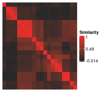
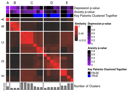
The clustering solutions are along the rows and columns of the above
figure, and the cells at the intersection between two solutions show how
similar they are to each other based on their ARI. The diagonals should
always be red, representing the maximum value of 1, as they show
self-similarity. Complete-linkage, Euclidean-distance based hierarchical
clustering is being applied to these solutions to obtain the row
ordering. This is also the default approach used by the
ComplexHeatmap package, the backbone of all heatmap
functions in metasnf.
This heatmap is integral to identifying the meta clusters created from your data using the space of parameters defined in the SNF config. We will later see how to further customize this heatmap to add in rich information about how each plotted cluster solution differs on various measures of quality, different clustering settings, and different levels of separation on input and out-of-model measures.
First, we’ll divide the heatmap into meta clusters by visual
inspection. The indices of our meta cluster boundaries can be passed
into the meta_cluster_heatmap function as the
split_vector parameter. You can determine this vector
either by trial and error (repeated replotting with different
split_vector values) or by using the
shiny_annotator function, a wrapper around functionality
from the InteractiveComplexHeatmap package.
While the shiny app is running, your R console will be unresponsive. Clicking on meta cluster cell boundaries and tracking the row/column indices (printed to the R console as well as displayed in the app) can get us the following vector:
A demonstration of the shiny app can be seen here: Meta Cluster Identification
shiny_annotator(ari_hm)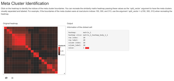
split_vec <- c(2, 5, 12, 17)This vector can be used to populate the meta cluster column in our solutions data frame as well as visualize our meta cluster boundaries more clearly.
mc_sol_df <- label_meta_clusters(
    sol_df,
    order = meta_cluster_order,
    split_vector = split_vec
)

mc_sol_df
#> 20 cluster solutions of 87 observations:
#> solution nclust mc uid_NDAR_INV0567T2Y9 uid_NDAR_INV0J4PYA5F
#>        1      5 E                     5                    2
#>        2      3 D                     3                    3
#>        3      9 C                     1                    7
#>        4      2 D                     1                    2
#>        5      8 C                     1                    6
#>        6      2 B                     1                    2
#>        7      4 C                     1                    4
#>        8      5 E                     3                    4
#>        9      3 D                     3                    3
#>       10      4 A                     2                    4
#> 10 solutions and 85 observations not shown.
#> Use `print(n = ...)` to change the number of rows printed.
#> Use `t()` to view compact cluster solution format.
ari_mc_hm <- meta_cluster_heatmap(
    sol_aris,
    order = meta_cluster_order,
    split_vector = split_vec
)

ari_mc_hm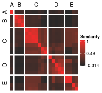
At this point, we have our meta clusters but are not yet sure of how they differ in terms of their structure across our input and out-of-model features.
Characterizing cluster solutions
Calculating associations between cluster solutions and initial data
We start by running the extend_solutions function, which
will calculate p-values representing the strength of the association
between cluster membership (treated as a categorical feature) and any
feature present in a provided data list and/or target_list.
extend_solutions also adds summary p-value measures
(min, mean, and max) of any features present in the target list. This
function can be quite slow depending on how large your data is; you can
monitor its progress by setting verbose = TRUE.
ext_sol_df <- extend_solutions(
    mc_sol_df,
    dl = input_dl,
    target_dl = target_dl
)

ext_sol_df
#> 20 cluster solutions, 87 observations, and p-values for 336 features.
#> Cluster assignment columns:
#> solution nclust mc uid_NDAR_INV0567T2Y9 uid_NDAR_INV0J4PYA5F
#> 1 5 E 5 2
#> 2 3 D 3 3
#> 3 9 C 1 7
#> 4 2 D 1 2
#> 5 8 C 1 6
#> 6 2 B 1 2
#> 7 4 C 1 4
#> 8 5 E 3 4
#> 9 3 D 3 3
#> 10 4 A 2 4
#> Association p-value columns:
#> solution mrisdp_1_pval mrisdp_2_pval mrisdp_3_pval mrisdp_4_pval
#> 1 4.0778e-01 8.7353e-01 1.8227e-01 6.4527e-01
#> 2 2.9963e-01 3.7253e-01 6.0899e-01 2.9392e-02
#> 3 2.4552e-01 2.2052e-01 1.1472e-01 5.2578e-01
#> 4 2.0034e-01 8.0738e-01 3.5087e-01 4.7769e-01
#> 5 1.8555e-01 4.5421e-01 1.0940e-01 4.5550e-01
#> 6 7.9908e-01 3.7914e-02 4.8240e-01 7.0521e-01
#> 7 4.7354e-01 3.7364e-01 1.0889e-01 8.1730e-01
#> 8 4.0837e-01 6.6968e-01 1.6713e-01 6.7935e-01
#> 9 2.5205e-01 3.4546e-01 3.6226e-01 1.4636e-02
#> 10 5.2398e-01 4.1312e-01 2.9576e-01 1.9681e-01
#> Summary p-value columns:
#> solution min_pval mean_pval max_pval
#> 1 7.263e-01 7.304e-01 7.344e-01
#> 2 3.238e-01 4.941e-01 6.644e-01
#> 3 3.961e-01 5.389e-01 6.817e-01
#> 4 4.844e-01 6.204e-01 7.564e-01
#> 5 2.257e-01 5.076e-01 7.895e-01
#> 6 1.325e-01 1.946e-01 2.566e-01
#> 7 1.230e-01 2.031e-01 2.832e-01
#> 8 7.112e-01 7.380e-01 7.648e-01
#> 9 5.110e-01 6.856e-01 8.602e-01
#> 10 1.034e-02 1.833e-02 2.631e-02
#> Summaries calculated from 2 features. Use `summary_features(x)` to see them.
#> 10 solutions and 332 features not shown.
#> Use `print(n = ...)` to change the number of rows printed.
#> Use `t()` to view compact cluster solution format.The difference between the data list passed into the dl
parameter and the one passed into the target_dl parameter
is that the target_dl features are the only ones used for
generating the p-value summary columns.
# No features are used to calculate summary p-values
ext_sol_df_no_summaries <- extend_solutions(
    mc_sol_df,
    dl = c(input_dl, target_dl)
)

# Every features are used to calculate summary p-values
ext_sol_df_all_summaries <- extend_solutions(
    mc_sol_df,
    target_dl = c(input_dl, target_dl)
)
Visualizing feature associations with meta clustering results
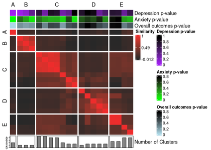
This ext_sol_df we created can be converted into a
standard data frame and passed into the
meta_cluster_heatmap function to easily visualize the level
of separation on each of our features for each of our cluster
solutions.
annotated_ari_hm <- meta_cluster_heatmap(
    sol_aris,
    order = meta_cluster_order,
    split_vector = split_vec,
    data = as.data.frame(ext_sol_df),
    top_hm = list(
        "Depression p-value" = "cbcl_depress_r_pval",
        "Anxiety p-value" = "cbcl_anxiety_r_pval",
        "Overall outcomes p-value" = "mean_pval"
    ),
    bottom_bar = list(
        "Number of Clusters" = "nclust"
    ),
    annotation_colours = list(
        "Depression p-value" = colour_scale(
            ext_sol_df$"cbcl_depress_r_pval",
            min_colour = "purple",
            max_colour = "black"
        ),
        "Anxiety p-value" = colour_scale(
            ext_sol_df$"cbcl_anxiety_r_pval",
            min_colour = "green",
            max_colour = "black"
        ),
        "Overall outcomes p-value" = colour_scale(
            ext_sol_df$"mean_pval",
            min_colour = "lightblue",
            max_colour = "black"
        )
    )
)
The meta_cluster_heatmap function wraps around a more
generic similarity_matrix_heatmap function in this package,
which itself is a wrapper around ComplexHeatmap::Heatmap().
Consequently, any parameter that can be used with
ComplexHeatmap::Heatmap() package can be used here. This
also makes the documentation for the ComplexHeatmap package
one of the best places to learn more about what can be done for further
customizing these heatmaps.
The data for the annotations don’t necessarily need to come from
functions in metasnf. For example, to highlight the
solutions where two very specific observations happened to cluster
together, we can easily add that information in as another annotation.
By converting an ext_solutions_df class object into a data
frame with the parameter keep_attributes = TRUE, the
resulting data frame will retain the p-value information from the
ext_solutions_df side of things, cluster assignment columns
from the solutions_df side of things, and
settings_df and weights_matrix columns from
the embedded original SNF config.
Then, we can use dplyr::mutate() to create a new column
flagging when two observations co-cluster.
annotation_data <- ext_sol_df |>
    as.data.frame(keep_attributes = TRUE) |>
    dplyr::mutate(
        key_subjects_cluster_together = dplyr::case_when(
            uid_NDAR_INVLF3TNDUZ == uid_NDAR_INVLDQH8ATK ~ TRUE,
            TRUE ~ FALSE
        )
    )

annotated_ari_hm2 <- meta_cluster_heatmap(
    sol_aris,
    order = meta_cluster_order,
    split_vector = split_vec,
    data = annotation_data,
    top_hm = list(
        "Depression p-value" = "cbcl_depress_r_pval",
        "Anxiety p-value" = "cbcl_anxiety_r_pval",
        "Key Subjects Clustered Together" = "key_subjects_cluster_together"
    ),
    bottom_bar = list(
        "Number of Clusters" = "nclust"
    ),
    annotation_colours = list(
        "Depression p-value" = colour_scale(
            ext_sol_df$"cbcl_depress_r_pval",
            min_colour = "purple",
            max_colour = "black"
        ),
        "Anxiety p-value" = colour_scale(
            ext_sol_df$"cbcl_anxiety_r_pval",
            min_colour = "purple",
            max_colour = "black"
        ),
        "Key Subjects Clustered Together" = c(
            "TRUE" = "blue",
            "FALSE" = "black"
        )
    )
)
Characterizing individual solutions representative of each meta cluster
Now that we’ve visually delineated our meta clusters, we can get a quick summary of what sort of separation exists across our input and held out features by taking a closer look at one representative cluster solution from each meta cluster.
This can be achieved by the get_representative_solutions
function, which extracts one cluster solution per meta cluster based on
having the highest average ARI with the other solutions in that meta
cluster.
rep_solutions <- get_representative_solutions(sol_aris, ext_sol_df)

mc_manhattan <- mc_manhattan_plot(
    rep_solutions,
    dl = input_dl,
    target_dl = target_dl,
    hide_x_labels = TRUE,
    point_size = 2,
    text_size = 12,
    threshold = 0.05,
    neg_log_pval_thresh = 5
)
neg_log_pval_thresh sets a threshold for the negative
log of the p-values to be displayed. At a value of 5, any p-value that
is smaller than 1e-5 will be truncated to 1e-5.
The plot as it is is a bit unwieldy plot given how many neuroimaging ROIs are present. Let’s take out the cortical thickness and surface area measures to make the plot a little clearer.
We’ll also be able to read some feature measures more clearly when we dial the number of features plotted back a bit, as well.
rep_solutions_no_cort <- dplyr::select(rep_solutions, -dplyr::contains("mrisdp"))

mc_manhattan2 <- mc_manhattan_plot(
    ext_sol_df = rep_solutions_no_cort,
    dl = input_dl,
    target_dl = target_dl,
    point_size = 4,
    threshold = 0.01,
    text_size = 12,
    domain_colours = c(
        "neuroimaging" = "cadetblue",
        "demographics" = "purple",
        "behaviour" = "firebrick"
    )
)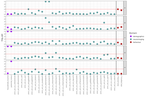
Note that the Manhattan plot automatically uses a vertical line to
separate features in the data_list argument from those in the
target_list. Vertical boundaries can be controlled with the
xints parameter.
Relating results to metasnf hyperparameters
If you see something interesting in your heatmap, you may be curious to know how that corresponds to the settings that were in your settings data frame.
You could certainly stack on each setting to the ARI heatmap as
annotations, but that may be a bit cumbersome given how many settings
there are. Another option is to start by taking a first look at entire
settings_df, sorted by the meta cluster results, through
the settings_df_heatmap function. The settings can be
passed in through either an snf_config or
settings_df class object.
config_hm <- config_heatmap(
    my_sc,
    order = meta_cluster_order,
    hide_fixed = TRUE
)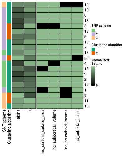
This heatmap rescales all the columns in the settings_df to have a
maximum value of 1. The purpose of re-ordering the settings data frame
in this way is to see if any associations exist between certain settings
values and pairwise cluster solution similarities. If there are any
particular important settings, you can simply add them into your
adjusted rand index heatmap annotations. Recall that the
solutions_df class (and, by extension, the
ext_solutions_df class that contains a
solutions_df object as an attribute) contain the SNF config
as an attribute, so no further data manipulation is needed to add a
setting as a heatmap annotation.
Give it a try with the code below:
annotation_data <- ext_sol_df |>
    as.data.frame(keep_attributes = TRUE) |>
    dplyr::mutate(
        key_subjects_cluster_together = dplyr::case_when(
            uid_NDAR_INVLF3TNDUZ == uid_NDAR_INVLDQH8ATK ~ TRUE,
            TRUE ~ FALSE
        )
    )

annotation_data$"clust_alg" <- as.factor(annotation_data$"clust_alg")

annotated_ari_hm3 <- meta_cluster_heatmap(
    sol_aris,
    order = meta_cluster_order,
    split_vector = split_vec,
    data = annotation_data,
    top_hm = list(
        "Depression p-value" = "cbcl_depress_r_pval",
        "Anxiety p-value" = "cbcl_anxiety_r_pval",
        "Key Subjects Clustered Together" = "key_subjects_cluster_together"
    ),
    left_hm = list(
        "Clustering Algorithm" = "clust_alg" # from the original settings
    ),
    bottom_bar = list(
        "Number of Clusters" = "nclust" # also from the original settings
    ),
    annotation_colours = list(
        "Depression p-value" = colour_scale(
            ext_sol_df$"cbcl_depress_r_pval",
            min_colour = "purple",
            max_colour = "black"
        ),
        "Anxiety p-value" = colour_scale(
            ext_sol_df$"cbcl_anxiety_r_pval",
            min_colour = "purple",
            max_colour = "black"
        ),
        "Key Subjects Clustered Together" = c(
            "TRUE" = "blue",
            "FALSE" = "black"
        )
    )
)

annotated_ari_hm3
Quality measures
Quality metrics are another useful heuristic for the goodness of a
cluster that don’t require any contextualization of results in the
domain they may be used in. metasnf enables measures of silhouette
scores, Dunn indices, and Davies-Bouldin indices. To calculate these
values, we’ll need not only the cluster results but also the final fused
network (the similarity matrices produced by SNF) that the clusters came
from. These similarity matrices can be collected from the
batch_snf using the return_sim_mats
parameter:
sol_df <- batch_snf(dl = input_dl, sc = my_sc, return_sim_mats = TRUE)Now, the solutions data frame contains a non-empty list of similarity matrices as one of its attributes. These similarity matrices are the final SNF-derived networks from each SNF run. Using that attribute, we can calculate the above mentioned quality metrics:
silhouette_scores <- calculate_silhouettes(sol_df)
dunn_indices <- calculate_dunn_indices(sol_df)
db_indices <- calculate_db_indices(sol_df)
Silhouette scores are calculated using the function
cluster::silhouette.
You can learn more about these functions here:
Stability measures
metasnf offers tools to evaluate two different measures of stability:
- Pairwise adjusted Rand indices (across resamplings of the clustering, on average, how similar was every pair of solutions according to the adjusted Rand index?)
- Fraction clustered together (what is the average fraction of times that observations who clustered together in the full results clustered together in resampled results?)
You can learn more about running stability calculations in the stability and coclustering vignette.
Evaluating separation across “target features” of importance
If you can specify a metric or objective function that may tell you how useful a clustering solution will be for your purposes in advance, that makes the cluster selection process much less arbitrary.
There are many ways to go about doing this, but this package offers
one way through a target_list. The target_list
contains data frames what we can examine our clustering results over
through linear regression (continuous data), ordinal regression (ordinal
data), or the Chi-squared test (categorical data).
Just like when generating the initial data_list, we need
to specify the name of the column in the provided data frames that is
originally being used to uniquely identify the different observations
from each other with the uid parameter.
We will next extend our sol_df with p-values from
regressing the target_list features onto our generated
clusters.
ext_sol_df <- extend_solutions(sol_df, target_dl)There is a heatmap for visualizing this too:
pval_hm <- pval_heatmap(ext_sol_df, order = meta_cluster_order)

pval_hm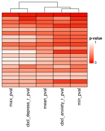
These p-values hold no real meaning for the traditional hypothesis-testing context, but they are reasonable proxies of the magnitude of the effect size / separation of the clusters across the features in question. Here, they are just a tool to find clustering solutions that are well-separated according to the outcome measures you’ve specified. Finding a cluster solution like this is similar to a supervised learning approach, but where the optimization method is just random sampling. The risk for overfitting your data with this approach is considerable, so make sure you have some rigorous external validation before reporting your findings.
We recommend using label propagation (provided by the
SNFtool package in the groupPredict function) for
validation: take the top clustering solutions found in some training
data, assign predicted clusters to some held out test observations, and
then characterize those test observations to see how well the clustering
solution seemed to have worked.
Validating results with label propagation
Here’s a quick step through of the complete procedure, from the beginning, with label propagation to validate our findings.
The metasnf package comes equipped with the function
train_test_assign to provide random splitting for you.
# All the observations present in all data frames with no NAs
all_observations <- uids(input_dl)

all_observations
#>  [1] "uid_NDAR_INV0567T2Y9" "uid_NDAR_INV0J4PYA5F" "uid_NDAR_INV10OMKVLE"
#>  [4] "uid_NDAR_INV15FPCW4O" "uid_NDAR_INV19NB4RJK" "uid_NDAR_INV1HLGR738"
#>  [7] "uid_NDAR_INV1KR0EZFU" "uid_NDAR_INV1L3Y9EOP" "uid_NDAR_INV1TCP5GNM"
#> [10] "uid_NDAR_INV1ZHRDJ6B" "uid_NDAR_INV2EJ41YSZ" "uid_NDAR_INV2PK6C85M"
#> [13] "uid_NDAR_INV2XO1PHCT" "uid_NDAR_INV3CU5Y9BZ" "uid_NDAR_INV3MBSY16V"
#> [16] "uid_NDAR_INV3N0QFDLO" "uid_NDAR_INV3N1476QE" "uid_NDAR_INV3Y027GVK"
#> [19] "uid_NDAR_INV40Z7GVYJ" "uid_NDAR_INV49UPOXHJ" "uid_NDAR_INV4N5XGZE8"
#> [22] "uid_NDAR_INV4OWRB536" "uid_NDAR_INV4X80QUZY" "uid_NDAR_INV50JL2RXP"
#> [25] "uid_NDAR_INV5BRNFYQC" "uid_NDAR_INV64F9GH0V" "uid_NDAR_INV6RVH5KZS"
#> [28] "uid_NDAR_INV6WBQCY2I" "uid_NDAR_INV752EFAQ0" "uid_NDAR_INV7O30HFV6"
#> [31] "uid_NDAR_INV7QO93CJH" "uid_NDAR_INV84G9ONXP" "uid_NDAR_INV8EHP6W1U"
#> [34] "uid_NDAR_INV8MJFUKIW" "uid_NDAR_INV8WGK6ECZ" "uid_NDAR_INV94AKNGMJ"
#> [37] "uid_NDAR_INV9GAZYV8Q" "uid_NDAR_INV9IREH05N" "uid_NDAR_INV9KC3GVMU"
#> [40] "uid_NDAR_INV9NFKZ82A" "uid_NDAR_INV9S1BMDE5" "uid_NDAR_INVA68OU0YK"
#> [43] "uid_NDAR_INVADCYZ38B" "uid_NDAR_INVAYM8WTIN" "uid_NDAR_INVB8O4LAQV"
#> [46] "uid_NDAR_INVBAP80W1R" "uid_NDAR_INVBTRW1NUK" "uid_NDAR_INVCIXE0496"
#> [49] "uid_NDAR_INVCYBSZD0N" "uid_NDAR_INVD37Z9N61" "uid_NDAR_INVD61ZUBC7"
#> [52] "uid_NDAR_INVDXKG2UBF" "uid_NDAR_INVEQ1OBNSM" "uid_NDAR_INVEQ4D2M8P"
#> [55] "uid_NDAR_INVEVBDLSTM" "uid_NDAR_INVEY0FMJDI" "uid_NDAR_INVFLU0YINE"
#> [58] "uid_NDAR_INVFNZPWMSI" "uid_NDAR_INVFY76P8AJ" "uid_NDAR_INVG3T0PXW6"
#> [61] "uid_NDAR_INVG5CI7XK4" "uid_NDAR_INVG8BRLSO9" "uid_NDAR_INVGDBYXWV4"
#> [64] "uid_NDAR_INVH1KV76BQ" "uid_NDAR_INVH3P4T8C2" "uid_NDAR_INVH4FZC2XB"
#> [67] "uid_NDAR_INVH8QN7WLT" "uid_NDAR_INVHERPS382" "uid_NDAR_INVHEUWA52I"
#> [70] "uid_NDAR_INVHM3XS68O" "uid_NDAR_INVI1RKT9MX" "uid_NDAR_INVIZFV08RU"
#> [73] "uid_NDAR_INVJ574KX6A" "uid_NDAR_INVK3FL5CP2" "uid_NDAR_INVK9ULDQA2"
#> [76] "uid_NDAR_INVKB0CYO1H" "uid_NDAR_INVKHWS26UN" "uid_NDAR_INVKTUMPLXY"
#> [79] "uid_NDAR_INVKYH529RD" "uid_NDAR_INVL4NIUZYF" "uid_NDAR_INVLDQH8ATK"
#> [82] "uid_NDAR_INVLF3TNDUZ" "uid_NDAR_INVLI58ERQC" "uid_NDAR_INVLIQRM8KC"
#> [85] "uid_NDAR_INVLXDP1SWT" "uid_NDAR_INVMBOZVEA4" "uid_NDAR_INVMIWOSHJN"

# Remove the "uid_" prefix to allow merges with the original data
all_observations <- gsub("uid_", "", all_observations)

# data frame assigning 80% of observations to train and 20% to test
assigned_splits <- train_test_assign(train_frac = 0.8, uids = all_observations)

# Pulling the training and testing observations specifically
train_obs <- assigned_splits$"train"
test_obs <- assigned_splits$"test"

# Partition a training set
train_cort_t <- cort_t[cort_t$"unique_id" %in% train_obs, ]
train_cort_sa <- cort_sa[cort_sa$"unique_id" %in% train_obs, ]
train_subc_v <- subc_v[subc_v$"unique_id" %in% train_obs, ]
train_income <- income[income$"unique_id" %in% train_obs, ]
train_pubertal <- pubertal[pubertal$"unique_id" %in% train_obs, ]
train_anxiety <- anxiety[anxiety$"unique_id" %in% train_obs, ]
train_depress <- depress[depress$"unique_id" %in% train_obs, ]

# Partition a test set
test_cort_t <- cort_t[cort_t$"unique_id" %in% test_obs, ]
test_cort_sa <- cort_sa[cort_sa$"unique_id" %in% test_obs, ]
test_subc_v <- subc_v[subc_v$"unique_id" %in% test_obs, ]
test_income <- income[income$"unique_id" %in% test_obs, ]
test_pubertal <- pubertal[pubertal$"unique_id" %in% test_obs, ]
test_anxiety <- anxiety[anxiety$"unique_id" %in% test_obs, ]
test_depress <- depress[depress$"unique_id" %in% test_obs, ]

# A data list with just training observations
train_dl <- data_list(
    list(train_cort_t, "cortical_thickness", "neuroimaging", "continuous"),
    list(train_cort_sa, "cortical_sa", "neuroimaging", "continuous"),
    list(train_subc_v, "subcortical_volume", "neuroimaging", "continuous"),
    list(train_income, "household_income", "demographics", "continuous"),
    list(train_pubertal, "pubertal_status", "demographics", "continuous"),
    uid = "unique_id"
)

# A data list with training and testing observations
full_dl <- data_list(
    list(cort_t, "cortical_thickness", "neuroimaging", "continuous"),
    list(cort_sa, "cortical_surface_area", "neuroimaging", "continuous"),
    list(subc_v, "subcortical_volume", "neuroimaging", "continuous"),
    list(income, "household_income", "demographics", "continuous"),
    list(pubertal, "pubertal_status", "demographics", "continuous"),
    uid = "unique_id"
)

# Construct the target lists
train_target_dl <- data_list(
    list(train_anxiety, "anxiety", "behaviour", "ordinal"),
    list(train_depress, "depressed", "behaviour", "ordinal"),
    uid = "unique_id"
)
# Find a clustering solution in your training data
set.seed(42)
my_sc <- snf_config(
    train_dl,
    n_solutions = 5,
    min_k = 10,
    max_k = 30
)

train_sol_df <- batch_snf(
    train_dl,
    my_sc
)

ext_sol_df <- extend_solutions(
    train_sol_df,
    train_target_dl
)
# The first row had the lowest minimum p-value across our outcomes
lowest_min_pval <- min(ext_sol_df$"min_pval")
which(ext_sol_df$"min_pval" == lowest_min_pval)
#> [1] 1

# Keep track of your top solution
top_row <- ext_sol_df[1, ]

# Use the solutions data frame from the training observations and the data list from
# the training and testing observations to propagate labels to the test observations
propagated_labels <- label_propagate(top_row, full_dl)

head(propagated_labels)
#>                    uid     group 1
#> 1 uid_NDAR_INV0567T2Y9 clustered 1
#> 2 uid_NDAR_INV0J4PYA5F clustered 2
#> 3 uid_NDAR_INV10OMKVLE clustered 1
#> 4 uid_NDAR_INV15FPCW4O clustered 1
#> 5 uid_NDAR_INV19NB4RJK clustered 1
#> 6 uid_NDAR_INV1HLGR738 clustered 1
tail(propagated_labels)
#>                     uid       group 1
#> 82 uid_NDAR_INVG5CI7XK4 unclustered 1
#> 83 uid_NDAR_INVGDBYXWV4 unclustered 1
#> 84 uid_NDAR_INVHEUWA52I unclustered 2
#> 85 uid_NDAR_INVK9ULDQA2 unclustered 1
#> 86 uid_NDAR_INVKYH529RD unclustered 1
#> 87 uid_NDAR_INVLDQH8ATK unclustered 1
You could, if you wanted, see how all of your clustering solutions propagate to the test set, but that would mean reusing your test set and removing the protection against overfitting conferred by this procedure.
propagated_labels_all <- label_propagate(
    ext_sol_df,
    full_dl
)
That’s all!
If you have any questions, comments, suggestions, bugs, etc. feel free to post an issue at https://github.com/BRANCHlab/metasnf.
References
Caruana, Rich, Mohamed Elhawary, Nam Nguyen, and Casey Smith. 2006. “Meta Clustering.” In Sixth International Conference on Data Mining (ICDM’06), 107–18. https://doi.org/10.1109/ICDM.2006.103.
Wang, Bo, Aziz M. Mezlini, Feyyaz Demir, Marc Fiume, Zhuowen Tu, Michael Brudno, Benjamin Haibe-Kains, and Anna Goldenberg. 2014. “Similarity Network Fusion for Aggregating Data Types on a Genomic Scale.” Nature Methods 11 (3): 333–37. https://doi.org/10.1038/nmeth.2810.