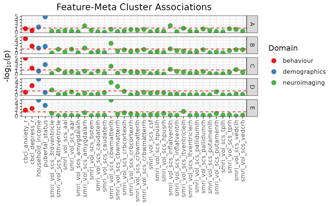
Manhattan plot of feature-meta cluster associaiton p-values

Given a data frame of representative meta cluster solutions (see get_representative_solutions(), returns a Manhattan plot for showing feature separation across all features in provided data/target lists.

Usage

mc_manhattan_plot(
  ext_sol_df,
  dl = NULL,
  target_dl = NULL,
  variable_order = NULL,
  neg_log_pval_thresh = 5,
  threshold = NULL,
  point_size = 5,
  text_size = 20,
  plot_title = NULL,
  xints = NULL,
  hide_x_labels = FALSE,
  domain_colours = NULL
)

Arguments

ext_sol_df

A sol_df that contains "_pval" columns containing the values to be plotted. This object is the output of extend_solutions().

dl

List of data frames containing data information.

target_dl

List of data frames containing target information.

variable_order

Order of features to be displayed in the plot.

neg_log_pval_thresh

Threshold for negative log p-values.

threshold

p-value threshold to plot horizontal dashed line at.

point_size

Size of points in the plot.

text_size

Size of text in the plot.

plot_title

Title of the plot.

xints

Either "outcomes" or a vector of numeric values to plot vertical lines at.

hide_x_labels

If TRUE, hides x-axis labels.

domain_colours

Named vector of colours for domains.

Value

A Manhattan plot (class "gg", "ggplot") showing the association p-values of features against each solution in the provided solutions data frame, stratified by meta cluster label.

Examples

# dl <- data_list(
#     list(subc_v, "subcortical_volume", "neuroimaging", "continuous"),
#     list(income, "household_income", "demographics", "continuous"),
#     list(pubertal, "pubertal_status", "demographics", "continuous"),
#     list(anxiety, "anxiety", "behaviour", "ordinal"),
#     list(depress, "depressed", "behaviour", "ordinal"),
#     uid = "unique_id"
# )
# 
# sc <- snf_config(
#     dl = dl,
#     n_solutions = 20,
#     min_k = 20,
#     max_k = 50
# )
# 
# sol_df <- batch_snf(dl, sc)
# 
# ext_sol_df <- extend_solutions(
#     sol_df,
#     dl = dl,
#     min_pval = 1e-10 # p-values below 1e-10 will be thresholded to 1e-10
# )
# 
# # Calculate pairwise similarities between cluster solutions
# sol_aris <- calc_aris(sol_df)
# 
# # Extract hierarchical clustering order of the cluster solutions
# meta_cluster_order <- get_matrix_order(sol_aris)
# 
# # Identify meta cluster boundaries with shiny app or trial and error
# # ari_hm <- meta_cluster_heatmap(sol_aris, order = meta_cluster_order)
# # shiny_annotator(ari_hm)
# 
# # Result of meta cluster examination
# split_vec <- c(2, 5, 12, 17)
# 
# ext_sol_df <- label_meta_clusters(ext_sol_df, split_vec, meta_cluster_order)
# 
# # Extracting representative solutions from each defined meta cluster
# rep_solutions <- get_representative_solutions(sol_aris, ext_sol_df)
# 
# mc_manhattan <- mc_manhattan_plot(
#     rep_solutions,
#     dl = dl,
#     point_size = 3,
#     text_size = 12,
#     plot_title = "Feature-Meta Cluster Associations",
#     threshold = 0.05,
#     neg_log_pval_thresh = 5
# )
# 
# mc_manhattan