Similarity Matrices

Download a copy of the vignette to follow along here: similarity_matrix_heatmaps.Rmd

This vignette walks through usage of similarity_matrix_heatmap to visualize the final similarity matrix produced by a run of SNF and how that matrix associates with other patient attributes.

Data set-up

library(metasnf)

# Generate data_list
data_list <- generate_data_list(
    list(
        data = expression_df,
        name = "expression_data",
        domain = "gene_expression",
        type = "continuous"
    ),
    list(
        data = methylation_df,
        name = "methylation_data",
        domain = "gene_methylation",
        type = "continuous"
    ),
    list(
        data = gender_df,
        name = "gender",
        domain = "demographics",
        type = "categorical"
    ),
    list(
        data = diagnosis_df,
        name = "diagnosis",
        domain = "clinical",
        type = "categorical"
    ),
    list(
        data = age_df,
        name = "age",
        domain = "demographics",
        type = "discrete"
    ),
    uid = "patient_id"
)

# Generate settings_matrix
settings_matrix <- generate_settings_matrix(
    data_list,
    nrow = 1,
    max_k = 40,
    seed = 42
)

## [1] "The global seed has been changed!"

# Run SNF and clustering
batch_snf_results <- batch_snf(
    data_list,
    settings_matrix,
    return_similarity_matrices = TRUE
)

## [1] "Row: 1/1 | Time remaining: 0 seconds"
## [1] "Total time taken: 0 seconds."

solutions_matrix <- batch_snf_results$"solutions_matrix"
similarity_matrices <- batch_snf_results$"similarity_matrices"

# The first (and only) similarity matrix:
similarity_matrix <- similarity_matrices[[1]]

# The first (and only) cluster solution:
cluster_solution <- get_cluster_solutions(solutions_matrix)$"1"

Visualize similarity matrices sorted by cluster label

similarity_matrix_heatmap is a wrapper for ComplexHeatmap::Heatmap, but with some convenient default transformations and parameters for viewing a similarity matrix.

similarity_matrix_hm <- similarity_matrix_heatmap(
    similarity_matrix = similarity_matrix,
    cluster_solution = cluster_solution,
    heatmap_height = grid::unit(10, "cm"),
    heatmap_width = grid::unit(10, "cm")
)

# Export heatmaps using the `save_heatmap` function
save_heatmap(
    heatmap = similarity_matrix_hm,
    path = "./similarity_matrix_heatmap.png",
    width = 410,
    height = 330,
    res = 80
)

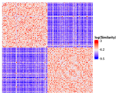
The default transformations include plotting log(Similarity) rather than the default similarity matrix as well as rescaling the diagonal of the matrix to the average value of the off-diagonals. Additionally, the similarity matrix gets reordered according to the provided cluster solution.

Annotations

One piece of functionality provided by ComplexHeatmap::Heatmap is the ability to supply visual annotations along the rows and columns of a heatmap.

You can always build annotations using the standard approaches outline in the ComplexHeatmap Complete Reference. In addition to that, this package offers some convenient functionality to specify regular heatmap annotations and barplot annotations directly through a provided dataframe or data_list (or both).

In the example below, we make use of data supplied through a data_list.

annotated_sm_hm <- similarity_matrix_heatmap(
    similarity_matrix = similarity_matrix,
    cluster_solution = cluster_solution,
    scale_diag = "mean",
    log_graph = TRUE,
    data_list = data_list,
    left_hm = list(
        "Diagnosis" = "diagnosis"
    ),
    top_hm = list(
        "Gender" = "gender"
    ),
    top_bar = list(
        "Age" = "age"
    ),
    annotation_colours = list(
        Diagnosis = c(
            "definite asthma" = "red3",
            "possible asthma" = "pink1",
            "no asthma" = "bisque1"
        ),
        Gender = c(
            "female" = "purple",
            "male" = "lightgreen"
        )
    ),
    heatmap_height = grid::unit(10, "cm"),
    heatmap_width = grid::unit(10, "cm")
)

save_heatmap(
    heatmap = annotated_sm_hm,
    path = "./annotated_sm_heatmap.png",
    width = 500,
    height = 440,
    res = 80
)

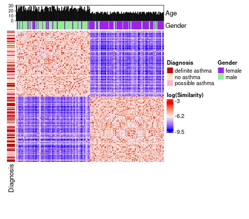
The colours red3, pink1, etc. are built-in R colours that you can browse by calling colours().

For reference, the code below shows how you would achieve these annotations using standard ComplexHeatmap syntax.

merged_df <- collapse_dl(data_list)
order <- sort(cluster_solution, index.return = TRUE)$"ix"
merged_df <- merged_df[order, ]

top_annotations <- ComplexHeatmap::HeatmapAnnotation(
    Age = ComplexHeatmap::anno_barplot(merged_df$"age"),
    Gender = merged_df$"gender",
    col = list(
        Gender = c(
            "female" = "purple",
            "male" = "lightgreen"
        )
    ),
    show_legend = TRUE
)

left_annotations <- ComplexHeatmap::rowAnnotation(
    Diagnosis = merged_df$"diagnosis",
    col = list(
        Diagnosis = c(
            "definite asthma" = "red3",
            "possible asthma" = "pink1",
            "no asthma" = "bisque1"
        )
    ),
    show_legend = TRUE
)

similarity_matrix_heatmap(
    similarity_matrix = similarity_matrix,
    cluster_solution = cluster_solution,
    scale_diag = "mean",
    log_graph = TRUE,
    data = merged_df,
    top_annotation = top_annotations,
    left_annotation = left_annotations
)

Take a look at the ComplexHeatmap Complete Reference to learn more about what is possible with this package.

More on sorting

Be aware that the ordering of both your data and your similarity matrix will be influenced if you supply values for the cluster_solution or order parameters. If you don’t think your data is lining up properly, consider manually making sure your similarity_matrix rows and columns are sorted to your preference (e.g., based on cluster) and that the order of your data matches. This will be easier to do with a dataframe than with a data_list, as the data_list forces patients to be sorted by their unique IDs upon generation.